twang package in R. We’ll also explore the importance of common support, the inverse probability weighting estimator (IPTW) and the double robust estimator, which combines a regression specification with a matching-based model in order to obtain a good estimate even when there is something wrong with one of the two underlying models.
Matching in R (III): Propensity Scores, Weighting (IPTW) and the Double Robust Estimator

In the last part of this series about Matching estimators in R, we’ll look at Propensity Scores as a way to solve covariate imbalance while handling the curse of dimensionality, and to how implement a Propensity Score estimator using the
Matching in R (II): Differences between Matching and Regression

Welcome to the second part of the series about Matching estimators in R. This sequel will build on top of the first part and the concepts explained there, so if you haven’t read it yet, I recommend doing so before you continue reading. But if you don’t have time for that, don’t worry. Here it’s a quick summary of the key ideas from the previous past that are required to understand this new post.
Matching in R (I): Subclassification, Common Support and the Curse of Dimensionality

Until this moment, the posts about causal inference on this blog have been centred around frameworks that enable the discussion of causal inference problems, such as Directed Acyclical Graphs (DAGs) and the Potential Outcomes model1. Now it’s time to go one step further and start talking about the “toolbox” that allows us to address causal inference questions when working with observational data (that is, data where the treatment variable is not under the full control of the researcher).
Randomization Inference in R: a better way to compute p-values in randomized experiments

Welcome to a new post of the series about the book Causal Inference: The Mixtape. In the previous post, we saw an introduction to the potential outcomes notation and how this notation allows us to express key concepts in the causal inference field.
One of those key concepts is that the simple difference in outcomes (SDO) is an unbiased estimator of the average treatment effect whenever the treatment has been randomly assigned (i.
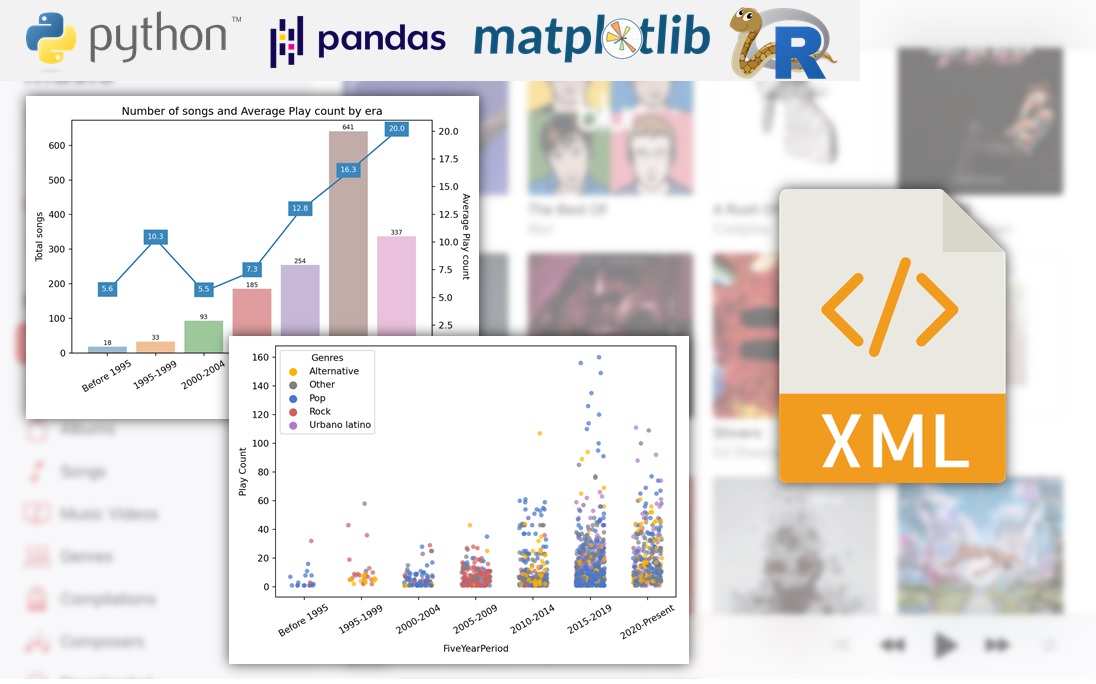
Analyzing my music collection with Python and R

A couple of months ago, I decided that it was time for me to finally grow out of my R comfort zone and start studying Python. I began my Python journey by reading the book Python for Data Analysis from Wes McKinney (creator of pandas, the Python equivalent of the tidyverse), and having finished it I wanted to put into practice what I’ve learned through an applied data analysis.