Randomization Inference in R: a better way to compute p-values in randomized experiments

Welcome to a new post of the series about the book Causal Inference: The Mixtape. In the previous post, we saw an introduction to the potential outcomes notation and how this notation allows us to express key concepts in the causal inference field.
One of those key concepts is that the simple difference in outcomes (SDO) is an unbiased estimator of the average treatment effect whenever the treatment has been randomly assigned (i.e., in those cases correlation is causation).
However, unbiasedness (having an expected value equal to the average effect) is not the only relevant property of a causal estimator. We’re also interested in the variance because, in the real world, we observe just individual realizations of the data generating process, which may as well be far away from the expected value1.
To incorporate this dimension in our analyses, we have tools such as means tests, linear regression, and the ANOVA, which take into consideration both the difference in means and the estimated variance to tell us how sure can we be about the existence of a true difference between treated and control units (i.e., about each group coming from a different data generating process).
These methods are very popular and their use is widespread, but this doesn’t mean they’re always the best tool for doing causal inference on experimental data. Because of that, today we’re going to talk about an alternative methodology which, under some circumstances, can be a better option to carry out hypothesis tests on randomized experiments. Its name is Randomization Inference.
Why bother?
A question you may be asking yourself at this point is why it would be worth investing time in learning and applying this methodology when we already have the usual hypothesis tests that are widely known and used. I would be asking myself the same.

The reasons to carry out hypothesis tests based on Randomization Inference (RI) can be summarised as follows:
When doing causal inference on experimental data, the main source of uncertainty is not the sampling from a bigger population but the random assignment of the treatment combined with the impossibility of knowing the counterfactual values. Standard hypotheses testing doesn’t take this into account and focuses on the sampling uncertainty instead. This is especially problematic if we work with large administrative datasets that literally represent “all the data” because it may lead to underestimating the total uncertainty in our figures. RI tackles this problem by considering the uncertainty that comes from the random assignment of the treatment, so it’s a better-suited methodology for these cases.
There are also advantages of using RI when we’re in the opposite situation: small data and/or very few treated units. In such cases, it doesn’t seem reasonable to rely on the “large samples” properties on which standard tests are based. Specifically, we may suffer from an increased vulnerability to outliers and high leverage observations, which translates to an increased risk of over-rejection of the null hypothesis. RI can help us in such situations because it’s a methodology more robust to outliers, especially when it is combined with ranking or quantile test statistics (which will be explained in detail later on).
Finally, even if there isn’t any particular problem with traditional hypothesis testing, RI gives us much more freedom regarding the statistics we can use. When using a standard hypothesis test, we’re restricted to statistics for which the variance can be estimated or the test has been constructed analytically. In contrast, RI allows us to use literally any scalar statistic that we can get from a dataset and it doesn’t even require us to assume a particular distribution function for its estimator. Some examples of useful statistics that we could use are quantile statistics (such as the median), ranking statistics, or the KS statistic (Kolmogorov-Smirnov) which measures differences the outcomes distributions.
As a bonus, doing Randomization Inference is cool, in the sense that in the causal inference world there is an aesthetic preference for placebo methodologies, and RI can be considered as one of them. These methodologies are characterised by simulating fake treatments in real data and then checking that we don’t find relevant effects for those fake treatments, so we can be more confident that the conclusions about the true treatment are valid2. Below we will see that RI does something very close to that.
Randomization Inference step by step in R
In order to explain the methodology itself, let’s remember first the goal and context on which we would apply this procedure. We’re analysing data coming from a randomized experiment and we have:
A set of observations that were randomly assigned to treatment and control groups.
An outcome variable (\(Y\)).
And we want to figure out if the treatment has any real effect over that outcome variable.
As there will always be differences between treatment and control groups (just because of the random variability in the data generating process), we need to carry out some hypothesis test to verify if the observed differences between groups are big enough to be considered as evidence of a causal effect.
When in this situation, we can perform a Randomization Inference hypothesis test by applying the following steps:
Step 1: choose a sharp null hypothesis
In a standard hypothesis test, we have a null hypothesis that states something regarding a population parameter, for instance, \(\beta_1=0\) where \(\beta_1\) is the coefficient of the treatment variable \(D\). What this null hypothesis is saying is that the average effect of the treatment is zero, but it doesn’t say anything about the individual treatment effects for each unit (\(\delta_i\)).
In contrast, when we do RI, we use a sharp null, that is, a null that says something about each one of the individual treatment effects (\(\delta_i\)).
The most used and well-known sharp null is the Fischer’s sharp null:
\[ \delta_i=0 \] Which posits that the treatment has zero effect for each of the units in the sample.
For the sake of simplicity, on this post we will use Fischer’s sharp null, but note that we may as well use alternative sharp nulls such as \(\delta_i=1\) or \(\delta_i=2\). We could even test sharp nulls in which different groups or units have different values of \(\delta_i\). All that is required is to have a null that states something about each \(\delta_i\), and not just about \(E[\delta_i]\).
Why would we want to use null hypotheses like these? Because it allows us to complete the missing potential outcomes values in our dataset.
The data we usually see in an experiment has this structure:
library(tidyverse)
library(magrittr)
library(causaldata)

ri <- causaldata::ri %>%
  mutate(id_unit = row_number(),
         y0 = as.numeric(y0),
         y1 = as.numeric(y1))

ri
## # A tibble: 8 × 6
## name d y y0 y1 id_unit
## <chr> <dbl> <dbl> <dbl> <dbl> <int>
## 1 Andy 1 10 NA 10 1
## 2 Ben 1 5 NA 5 2
## 3 Chad 1 16 NA 16 3
## 4 Daniel 1 3 NA 3 4
## 5 Edith 0 5 5 NA 5
## 6 Frank 0 7 7 NA 6
## 7 George 0 8 8 NA 7
## 8 Hank 0 10 10 NA 8For each unit, we observe both \(D_i\) and \(Y_i\), but just one of the potential outcomes (\(Y_i^0\) or \(Y_i^1\)). By leveraging the sharp null, we can fill in the missing values in the columns y0 and y1 (in this case, based on \(Y_i=Y_i^0=Y_i^1\)).
ri_fischer_null <- ri %>%
  mutate(y0 = y,
         y1 = y)

ri_fischer_null
## # A tibble: 8 × 6
## name d y y0 y1 id_unit
## <chr> <dbl> <dbl> <dbl> <dbl> <int>
## 1 Andy 1 10 10 10 1
## 2 Ben 1 5 5 5 2
## 3 Chad 1 16 16 16 3
## 4 Daniel 1 3 3 3 4
## 5 Edith 0 5 5 5 5
## 6 Frank 0 7 7 7 6
## 7 George 0 8 8 8 7
## 8 Hank 0 10 10 10 8Since we’re assuming that the treatment has an effect equal to zero for each unit, both potential outcomes are equal to the observed outcome.
Of course, we’re not claiming that this is really the case. We just want to discover how unlikely it is, under the sharp null assumption, to have observed the differences in means that we got in our experiment.
Step 2: pick a test statistic
To conduct a hypothesis test, we also need a statistic. In a standard hypothesis test, it would be necessary to use a statistic for which we had a variance estimator but, when doing RI, we can use literally any scalar statistic that can be obtained from a treatment assignments vector (\(D\)) and an outcomes vector (\(Y\)).
One of the simplest statistics we can use is the simple difference in mean outcomes (SDO) between groups.
# Function that defines the statistic: it receives a dataframe as input,
# with the columns `y` (outcome) and `d` (treatment assignment), and returns
# a scalar value
sdo <- function(data) {
  data %>%
    summarise(te1 = mean(y[d == 1]),
              te0 = mean(y[d == 0]),
              sdo = te1 - te0) %>%
    pull(sdo)
}

sdo(ri_fischer_null)
## [1] 1However, as I said before, there is no reason why we couldn’t use a different test statistic. This freedom is one of the main reasons for which we would want to do RI in the first place.
Some examples of alternative test statistics we could use are:
Quantile statistics, for example, the difference in medians (or any other percentile) between two groups. They’re particularly useful if we have problems with outliers or high leverage observations.
Ranking statistics, which transform an outcome variable (\(Y\)) into ranking values (1 for the lowest outcome, 2 for the second-lowest, and so on) and then compute a metric based on those rankings (for instance, the difference in mean or median ranking).
KS statistic (Kolmogorov-Smirnov), which detects differences between outcome distributions by measuring the maximum distance between the cumulative distribution functions. This statistic would allow us, for instance, to identify the effect of a treatment that changes the variance or dispersion of the outcome but not its mean.
For simplicity’s sake (again), the SDO will be used as test statistic in this example but, afterwards, I will show another code example using the KS statistic.
Step 3: simulate many treatment assignments to get the statistic distribution
The next step consists in getting the distribution of values that the test statistic may take under the sharp null.
For this:
We will do permutations over the vector \(D\) using the same random process that was used for obtaining the random treatment assignments in the first place. For example, if the treatment was assigned by a process equivalent to tossing a coin for each unit (\(B(n, 0.5)\)), then the permutations must be generated in the same way.3
In our example, the random process consists in drafting 4 treatment assignments for a sample of 8 observations, which translates to 70 possible permutations in total. The following code obtains such permutations:
perms <- t(combn(ri_fischer_null$id_unit, 4)) %>% asplit(1)

perms_df <-
  tibble(treated_units = perms) %>%
  transmute(id_perm = row_number(),
            treated_units = map(treated_units, unlist))

ri_permuted <-
  crossing(perms_df, ri_fischer_null) %>%
  mutate(d = map2_dbl(id_unit, treated_units, ~.x %in% .y))

ri_permuted
## # A tibble: 560 × 8 ## id_perm treated_units name d y y0 y1 id_unit ## <int> <list> <chr> <dbl> <dbl> <dbl> <dbl> <int> ## 1 1 <int [4]> Andy 1 10 10 10 1 ## 2 1 <int [4]> Ben 1 5 5 5 2 ## 3 1 <int [4]> Chad 1 16 16 16 3 ## 4 1 <int [4]> Daniel 1 3 3 3 4 ## 5 1 <int [4]> Edith 0 5 5 5 5 ## 6 1 <int [4]> Frank 0 7 7 7 6 ## 7 1 <int [4]> George 0 8 8 8 7 ## 8 1 <int [4]> Hank 0 10 10 10 8 ## 9 2 <int [4]> Andy 1 10 10 10 1 ## 10 2 <int [4]> Ben 1 5 5 5 2 ## # ℹ 550 more rowsri_permuted %>% pull(id_perm) %>% n_distinct()## [1] 70For each permutation, we simulate the values of \(Y\) based on the previously chosen sharp null and the now complete potential outcomes columns. For Fischer’s sharp null, we don’t have to do anything because it states that \(Y_i=Y_i^0=Y_i^1\), which leads to the vector \(Y\) remaining unchanged no matter the values in \(D\). However, if our sharp null was something like \(\delta_i=1\), then it would be necessary to update/change the values of \(Y\) in each permutation.
We compute the test statistic value (the SDO in our example) for each permutation and then save those values.
perms_stats <-
  ri_permuted %>%
  group_by(id_perm) %>%
  summarise(te1 = mean(y[d == 1]),
            te0 = mean(y[d == 0]),
            sdo = te1 - te0)

perms_stats %>%
  select(id_perm, sdo)
## # A tibble: 70 × 2 ## id_perm sdo ## <int> <dbl> ## 1 1 1 ## 2 2 2 ## 3 3 3 ## 4 4 3.5 ## 5 5 4.5 ## 6 6 -4.5 ## 7 7 -3.5 ## 8 8 -3 ## 9 9 -2 ## 10 10 -2.5 ## # ℹ 60 more rowsVoilà! The statistic values obtained in (3) tell us what the statistic’s distribution is under the sharp null assumption.
ggplot(perms_stats, aes(sdo)) +
  geom_histogram() +
  labs(x = "Test statistic (SDO)")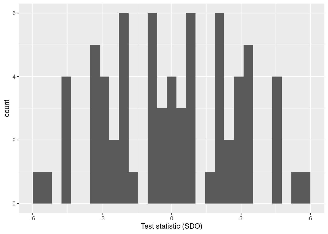
How many permutations should we do? Ideally, we should obtain all the possible permutations in order to get an exact representation of the test statistic distribution under the sharp null. However, this is only feasible in very small datasets: even with a dataset of 2000 rows, it becomes computationally prohibitive to get all the possible permutations of the treatment assignment.
The fall-back option, in this case, is to resign oneself to do enough permutations to get a reasonable approximation to the statistic’s distribution4.
Step 4: obtaining the p-value by comparing the “real” statistic with its simulated distribution
After having obtained the statistic’s distribution (exact or approximated) under the sharp null, we can proceed to locate the true statistic (the one that comes from the real values of \(D\) and \(Y\)) inside that distribution.
Note that if we want to perform a two-tailed test (the most common one), we must apply the absolute value function to the statistic distribution (which is, in fact, what we do in this example).
true_statistic <- perms_stats %>%
  filter(id_perm == 1) %>%
  pull(sdo)

ggplot(perms_stats,
       # Applying `abs` because we want a two tailed test
       aes(abs(sdo))) +
  geom_histogram() +
  labs(x = "Absolute value of the test statistic (SDO)",
       y = "count") +
  geom_vline(xintercept = true_statistic, colour = "red", size = 2) +
  annotate(geom = "label",
           x = true_statistic,
           y = 10,
           label = "'True' statistic",
           colour = "red") +
  annotate("segment", x = true_statistic+1, xend = true_statistic+3, y = 9, yend =9,
           colour = "purple", size = 2, arrow = arrow()) +
  annotate(geom = "label",
           x = true_statistic+2,
           y = 10,
           label = "More 'extreme' statistics",
           colour = "purple")
## Warning: Using `size` aesthetic for lines was deprecated in ggplot2 3.4.0.
## ℹ Please use `linewidth` instead.
## This warning is displayed once every 8 hours.
## Call `lifecycle::last_lifecycle_warnings()` to see where this warning was
## generated.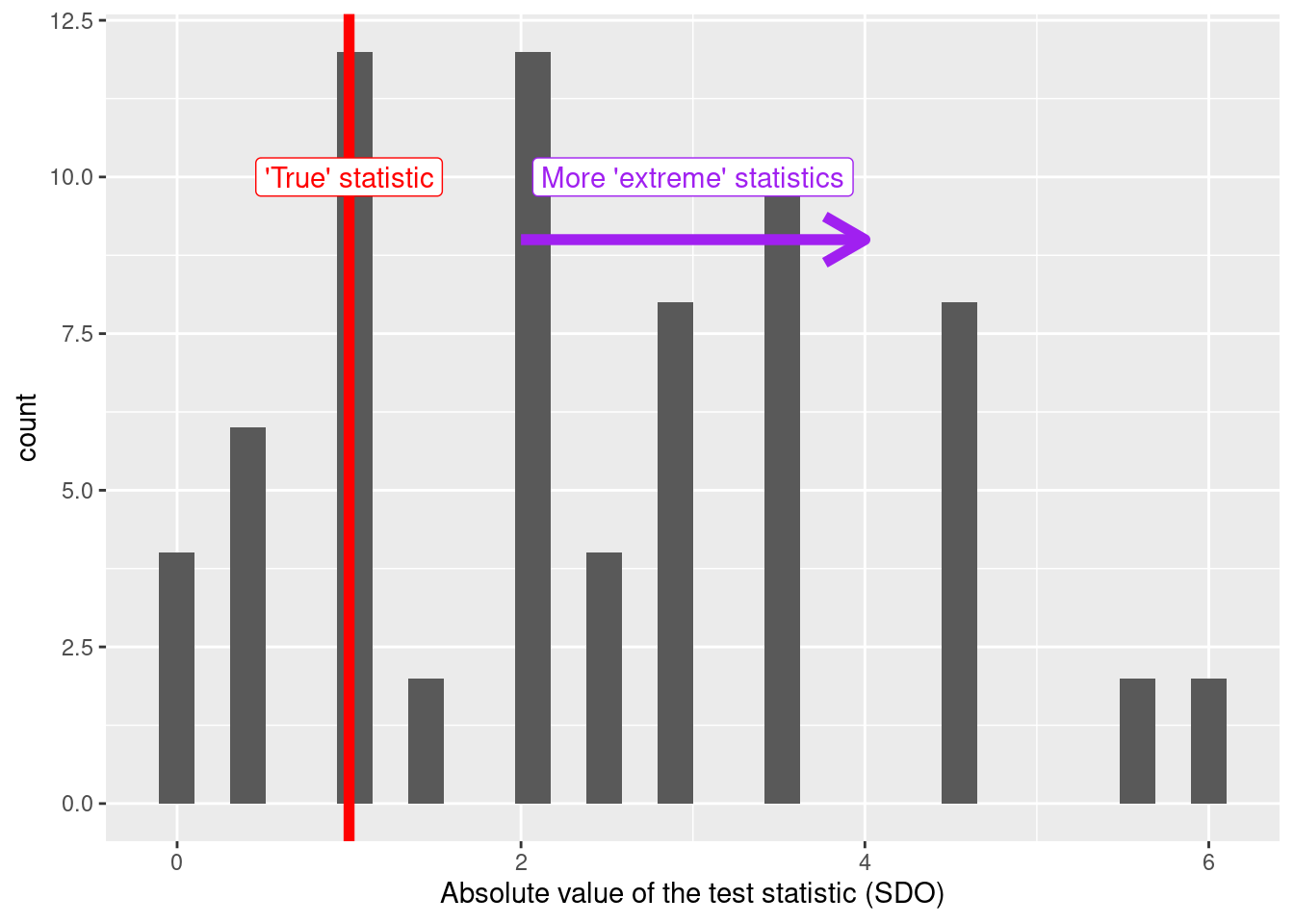
Having done this, we can calculate the p-value itself (which is what we have been looking for since the beginning).
This p-value can be calculated through the following steps:
- We create a descending ranking with the test statistics we obtained through the permutations (the highest value gets a ranking equal to 1, the lowest value gets a ranking equal to N). These rankings are assigned through a
row_number()-like algorithm. When there are ties, the original ranking of the tied statistics is replaced with the maximum ranking inside that group. For instance, if three statistics have the same value and their original rankings are 2, 3 and 4, all of them end up with a ranking equal to 4.
perms_ranked <- perms_stats %>%
  # Just like before, we apply `abs()` to get a two tailed test
  mutate(abs_sdo = abs(sdo)) %>%
  select(id_perm, abs_sdo) %>%
  arrange(desc(abs_sdo)) %>%
  mutate(rank = row_number(desc(abs_sdo))) %>%
  group_by(abs_sdo) %>%
  mutate(new_rank = max(rank))

perms_ranked
## # A tibble: 70 × 4
## # Groups: abs_sdo [11]
## id_perm abs_sdo rank new_rank
## <int> <dbl> <int> <int>
## 1 25 6 1 2
## 2 46 6 2 2
## 3 24 5.5 3 4
## 4 47 5.5 4 4
## 5 5 4.5 5 12
## 6 6 4.5 6 12
## 7 22 4.5 7 12
## 8 23 4.5 8 12
## 9 48 4.5 9 12
## 10 49 4.5 10 12
## # ℹ 60 more rows- We calculate the ratio between the final ranking of the true statistic and N, the total number of permutations we did.
n <- nrow(perms_ranked)

p_value <-
  perms_ranked %>%
  filter(id_perm == 1) %>%
  pull(new_rank)/n

p_value
## [1] 0.8571429In our example, the p-value we got is 0.86, which implies that we can’t reject the sharp null at a 5% significance level (in fact, we can’t reject it at any conventional significance level 😅). In other words, the SDO from the original data is not an unlikely value to observe if we assume that the treatment had zero effect on all the units and that the only source of variability in the statistic is the random assignment of \(D\).
Making it easier with the ri2 package 🤗
The R code shown above had the goal of explaining each step of the RI procedure. However, it’s not very concise and adapting it for other datasets would be tiresome and error prone. For that reason, it’s recommended to perform RI using one of the R packages that have been designed and developed for that end, such as ri2.
library(ri2)However, something from the “manual” code that doesn’t change is that we still have to provide 1) a test statistic, 2) a sharp null hypothesis, and 3) a randomization procedure. And just like before, the randomization procedure passed to ri2 must be the same as the one used for assigning the treatment in the first place.
The difference is that now we can pass these elements more in an easier and clearer way.
To declare the randomization procedure we use the function ri2::declare_ra. In this case (just like in the preceding example), we’re declaring the random assignment of 4 treatment units (m = 4) in a sample of 8 units (N = 8).
declaration <- declare_ra(N = 8, m = 4)
declaration
## Random assignment procedure: Complete random assignment
## Number of units: 8
## Number of treatment arms: 2
## The possible treatment categories are 0 and 1.
## The number of possible random assignments is 70.
## The probabilities of assignment are constant across units:
## prob_0 prob_1
## 0.5 0.5The output is stored in an R object that later we can pass to the function ri2::conduct_ri, which is the function that performs the RI procedure itself.
To declare the test statistic we have two options.
The first is to use the formula argument in the conduct_ri function. If our test statistic is just the SDO, then the formula will be something like y ~ d, where y is the outcome variable and d is the treatment assignment variable.
Alternatively, we can specify the statistic through the argument test_function (also in the function conduct_ri), which admits any R function capable of receiving a dataframe and returning a scalar (i.e., the statistic value).
In our example we’re going to use this last method:
# Declaring the `test_function`
sdo <- function(data) {
  # it receives a dataframe
  data %>%
  summarise(te1 = mean(y[d == 1], na.rm=TRUE),
            te0 = mean(y[d == 0], na.rm=TRUE),
            sdo = te1 - te0) %>%
    # and returns a scalar
    pull(sdo)
}
The sharp null hypothesis can be specified through the sharp_hypothesis argument in conduct_ri. The default value for this argument is 0, so if we’re going to use Fischer’s sharp null then we omit it in our code.
Last but not least, we have to indicate the names that the columns containing \(Y\) and \(D\) have in our data, using the assignment and outcome arguments, and we also have to pass the dataset itself through the argument data.
After specifying all those arguments, we can execute the function conduct_ri and then inspect the output with the summary.
ri2_out <- conduct_ri(
  test_function = sdo,
  assignment = "d",
  outcome = "y",
  declaration = declaration,
  sharp_hypothesis = 0,
  data = ri
)

summary(ri2_out)
## term estimate two_tailed_p_value
## 1 Custom Test Statistic 1 0.8571429As we see, the p-value returned by conduct_ri is exactly the same as the one we got with the “manual” code from the previous section, but now the code is much simpler and easier to read 😊.
Another advantage of conduct_ri is that its output can be directly plotted by the function plot().
plot(ri2_out)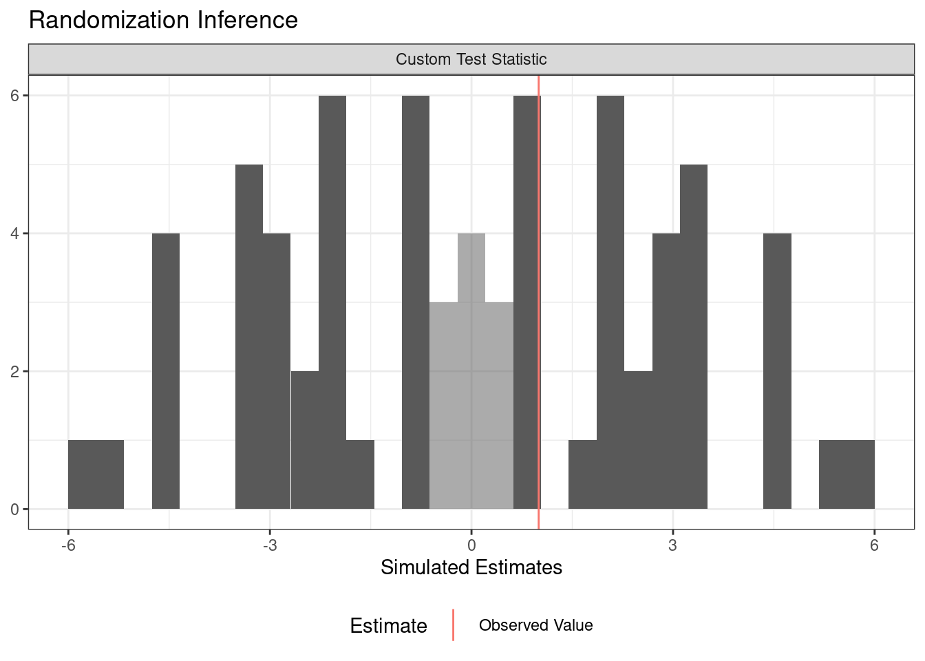
This plot is even better than the one we created manually in the previous section because it automatically highlights the statistics that are as or more extreme than the real statistic. It also appropriately portrays two-tailed tests without having to transform the statistics to their absolute value ✨.
In addition, since the output of plot(ri2_out) is a ggplot2 object, we can customize it or transform it through the ggplot2 functions we already know. For example, we can apply a ggthemes theme to make it look like a Stata plot:
plot(ri2_out) +
  ggthemes::theme_stata()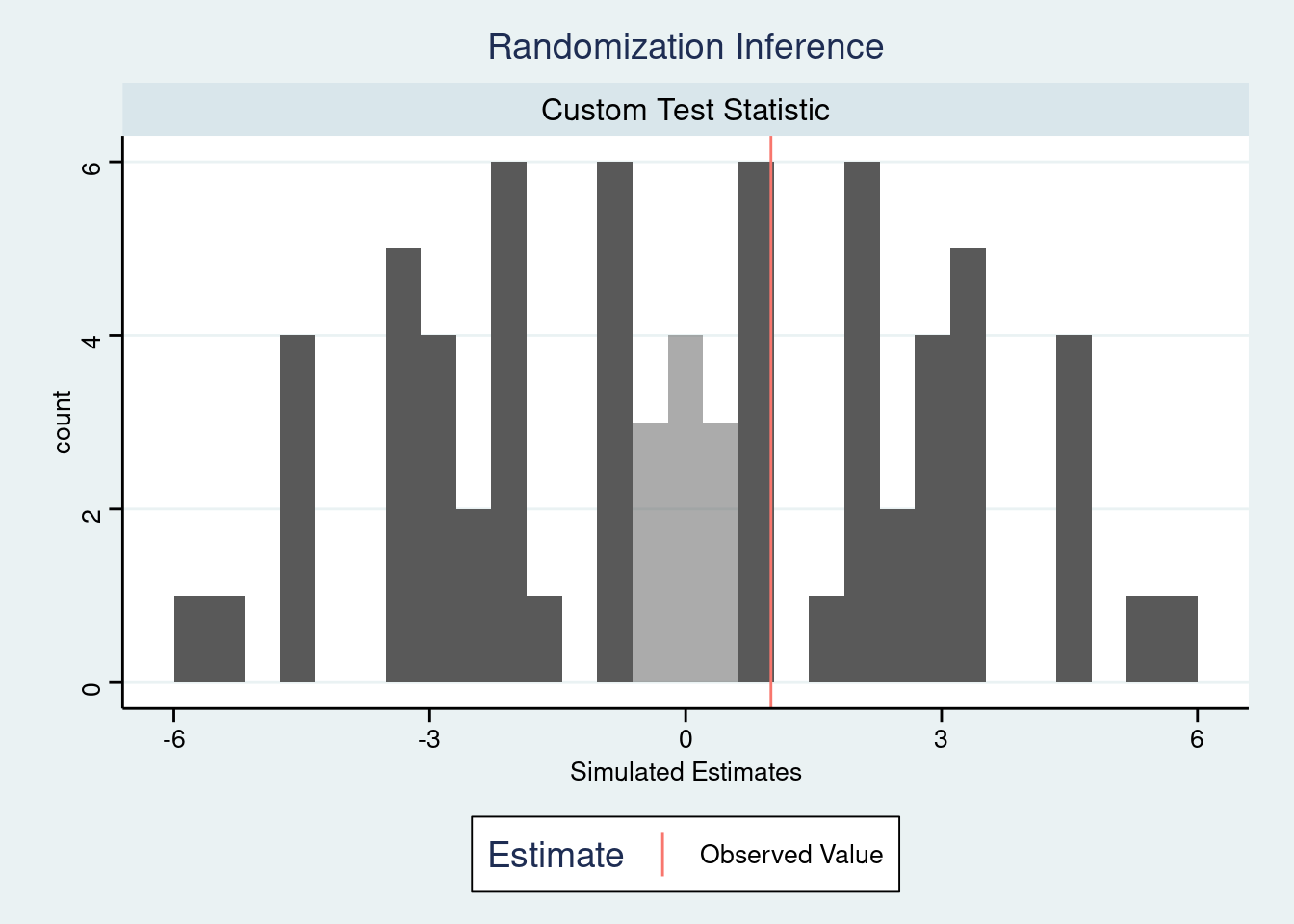
If we want to manually inspect the simulations data, we can extract the dataframe sims_df from the output of conduct_ri. This dataframe will have as many rows as permutations of \(D\) had been performed.
ri2_out[["sims_df"]] %>% head()## est_sim est_obs term
## 1 -1.0 1 Custom Test Statistic
## 2 -2.0 1 Custom Test Statistic
## 3 -3.0 1 Custom Test Statistic
## 4 -3.5 1 Custom Test Statistic
## 5 -4.5 1 Custom Test Statistic
## 6 4.5 1 Custom Test StatisticIt’s worth noting that conduct_ri also has a sims argument that specifies the number of permutations that will be carried out in order to obtain the p-value. Its default value is 1000, but we may want to increase it to get a more precise estimate.
Bonus: using the KS statistic to measure differences between outcome distributions
One of the advantages of RI that were mentioned at the beginning of this post was the freedom to use alternative test statistics, having as only restriction to be scalar values obtained from \(D\) and \(Y\).
One of the most interesting “alternative” statistics (in my opinion) is the KS statistic (Kolmogorov-Smirnov), which measures the maximum distance between two empirical cumulative distribution functions (ECDFs). In this case, it measures the distance between the ECDF of the treated units \(\hat{F_T}\) and the ECDF of the control units \(\hat{F_C}\):
\[ T_{KS}=\max|\hat{F_T}(Y_i) - \hat{F_C}(Y_i)| \]
We can see a visual example in the following plot, where the KS statistic equals the length of the red dotted line.

Example of KS statistic with 2 cumulative distribution functions. Source: StackExchange
Why would we use the KS statistic instead of something more familiar, like the difference in means?
Because we could have a treatment that affects the outcome distribution without changing the mean significantly. For instance, it could change the variance or generate a bi-modal distribution (translation into a real-world example: a treatment that has a large positive effect for half of the sample and a large negative effect for the other half).
Here is an example from the Mixtape with simulated data:
tb <- tibble(
  d = c(rep(0, 20), rep(1, 20)),
  y = c(0.22, -0.87, -2.39, -1.79, 0.37, -1.54,
        1.28, -0.31, -0.74, 1.72,
        0.38, -0.17, -0.62, -1.10, 0.30,
        0.15, 2.30, 0.19, -0.50, -0.9,
        -5.13, -2.19, 2.43, -3.83, 0.5,
        -3.25, 4.32, 1.63, 5.18, -0.43,
        7.11, 4.87, -3.10, -5.81, 3.76,
        6.31, 2.58, 0.07, 5.76, 3.50)
)

kdensity_d1 <- tb %>%
  filter(d == 1) %>%
  pull(y)
kdensity_d1 <- density(kdensity_d1)

kdensity_d0 <- tb %>%
  filter(d == 0) %>%
  pull(y)
kdensity_d0 <- density(kdensity_d0)

kdensity_d0 <- tibble(x = kdensity_d0$x, y = kdensity_d0$y, d = 0)
kdensity_d1 <- tibble(x = kdensity_d1$x, y = kdensity_d1$y, d = 1)

kdensity <- full_join(kdensity_d1, kdensity_d0,
                      by = c("x", "y", "d"))
kdensity$d <- as_factor(kdensity$d)

ggplot(kdensity)+
  geom_point(size = 0.3, aes(x,y, color = d))+
  xlim(-7, 8)+
  scale_color_discrete(labels = c("Control", "Treatment"))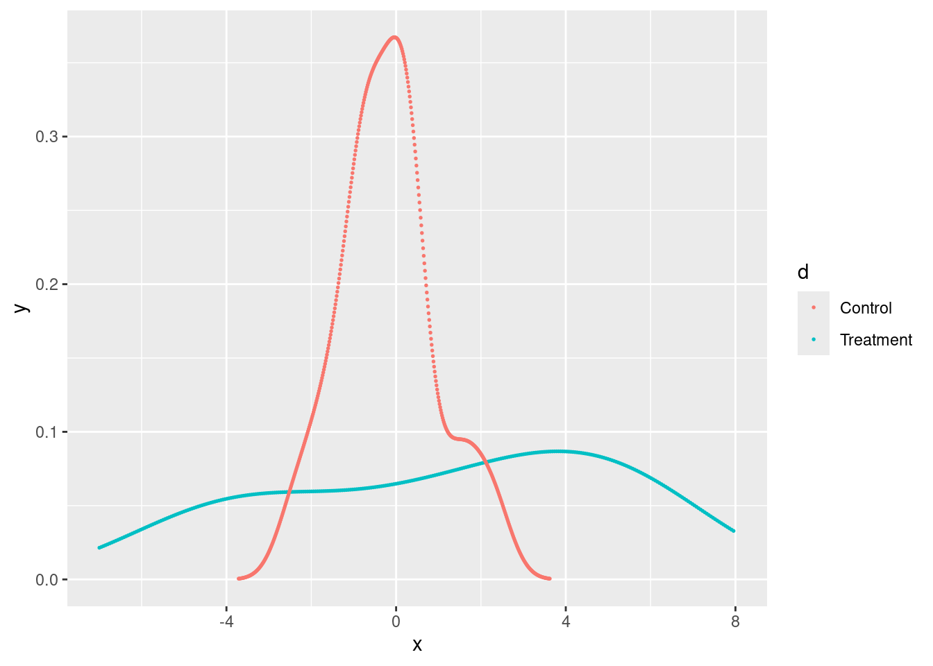
If we do RI with the data from above using the SDO as test statistic, we can’t reject the sharp null of having zero effect for all the units, despite having two evidently different outcome distributions.
set.seed(1989)

conduct_ri(
  test_function = sdo,
  assignment = "d",
  outcome = "y",
  declaration = declare_ra(N = 40, m = 20),
  sharp_hypothesis = 0,
  data = tb,
  sims = 10000
)
## term estimate two_tailed_p_value
## 1 Custom Test Statistic 1.415 0.1361Let’s see what happens if we use the KS statistic instead of the SDO:
# Declaring the function that obtains the KS statistic from a dataframe
ks_statistic <- function(data) {

  control <- data[data$d == 0, ]$y
  treated <- data[data$d == 1, ]$y

  cdf1 <- ecdf(control)
  cdf2 <- ecdf(treated)

  minMax <- seq(min(control, treated),
                max(control, treated),
                length.out=length(c(control, treated)))

  x0 <-
    minMax[which(abs(cdf1(minMax) - cdf2(minMax)) == max(abs(cdf1(minMax) - cdf2(minMax))))]

  y0 <- cdf1(x0)
  y1 <- cdf2(x0)

  diff <- unique(abs(y0 - y1))

  diff

}

# Obtaining the p-value through RI with the KS statistic
set.seed(1989)

ri_ks <-
  conduct_ri(
    test_function = ks_statistic,
    assignment = "d",
    outcome = "y",
    declaration = declare_ra(N = 40, m = 20),
    sharp_hypothesis = 0,
    data = tb,
    sims = 10000
  )

ri_ks
## term estimate two_tailed_p_value
## 1 Custom Test Statistic 0.45 0.0227The KS statistic does allow us to reject the sharp null at a 5% significance level5.
In the following plot, we can visualise the KS statistic corresponding to the true treatment assignment, along with the empirical CDFs of the treatment and control groups.
tb2 <- tb %>%
group_by(d) %>%
arrange(y) %>%
mutate(rn = row_number()) %>%
ungroup()


cdf1 <- ecdf(tb2[tb2$d == 0, ]$y)
cdf2 <- ecdf(tb2[tb2$d == 1, ]$y)

minMax <- seq(min(tb2$y),
              max(tb2$y),
              length.out=length(tb2$y))

x0 <-
  minMax[which(abs(cdf1(minMax) - cdf2(minMax)) == max(abs(cdf1(minMax) - cdf2(minMax))) )]

y0 <- cdf1(x0)
y1 <- cdf2(x0)

ggplot(tb2) +
  geom_step(aes(x=y, y=rn, color=factor(d)),
            size = 1.5, stat="ecdf") +
  labs(y = "Density") +
  geom_segment(aes(x = x0[1], y = y0[1], xend = x0[1], yend = y1[1]),
               linetype = "dashed", color = "red", size = 1) +
  geom_point(aes(x = x0[1] , y= y0[1]), color="red", size=4) +
  geom_point(aes(x = x0[1] , y= y1[1]), color="red", size=4)
## Warning in geom_segment(aes(x = x0[1], y = y0[1], xend = x0[1], yend = y1[1]), : All aesthetics have length 1, but the data has 40 rows.
## ℹ Did you mean to use `annotate()`?## Warning in geom_point(aes(x = x0[1], y = y0[1]), color = "red", size = 4): All aesthetics have length 1, but the data has 40 rows.
## ℹ Did you mean to use `annotate()`?## Warning in geom_point(aes(x = x0[1], y = y1[1]), color = "red", size = 4): All aesthetics have length 1, but the data has 40 rows.
## ℹ Did you mean to use `annotate()`?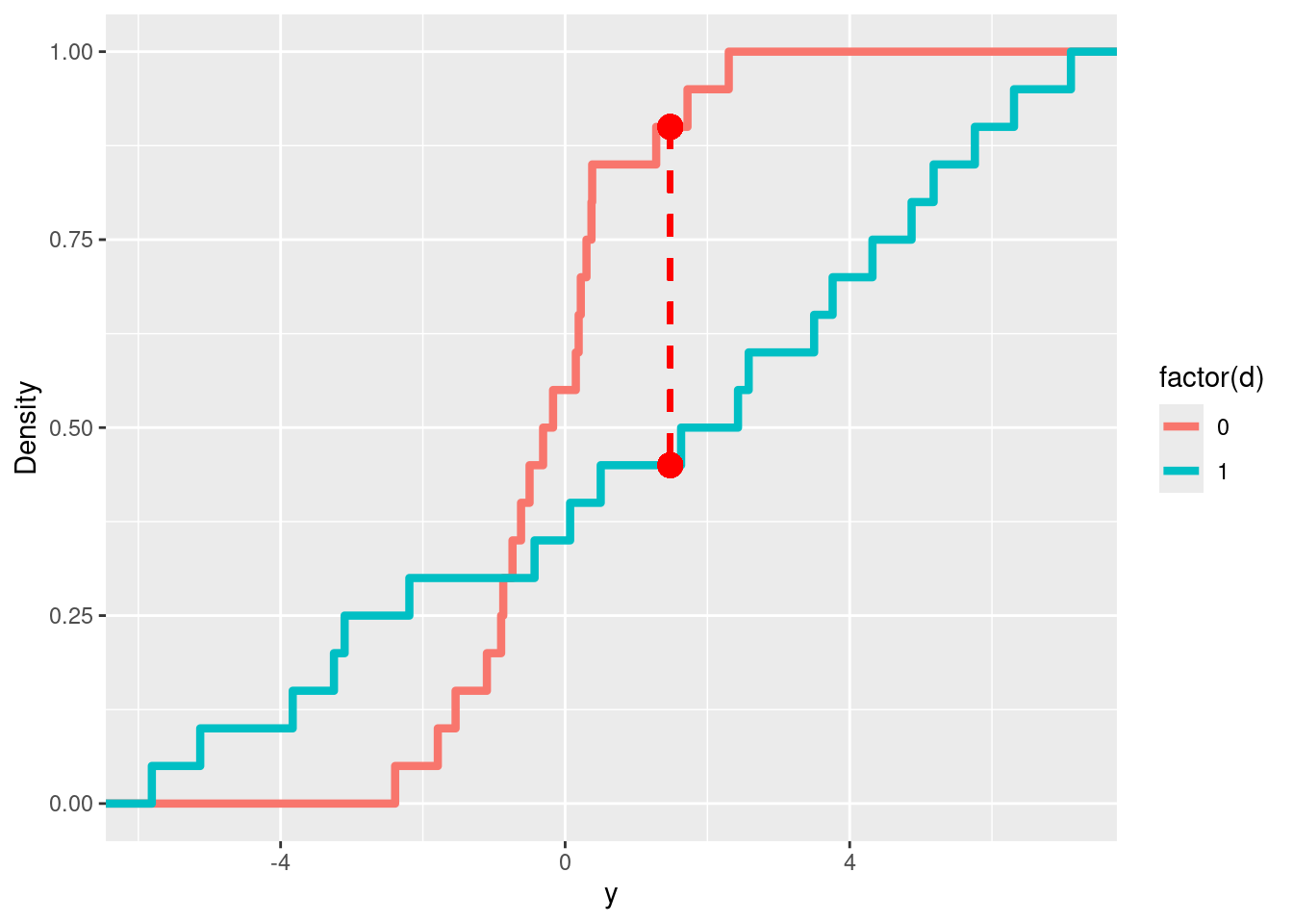
Considerations and additional references 🔍📚
To conclude, I would like to comment on some additional details and considerations regarding the RI methodology:
In order to obtain confidence intervals with RI we can iterate over a range of possible values for the test statistic and use each of them as sharp null in each iteration. The confidence interval will include all those values for which the sharp null couldn’t be rejected.
The Mixtape warns us that RI has some bias against small effects when it is used among Fischer’s sharp null. This is because only relatively large treatment effects will allow rejecting that null at conventional significance levels (small effects would be “swamped by the randomization process”). Therefore, if we expect the treatment effect to be small, we should either add covariates that explain the outcome variable (we can do that with the argument
formulainri2::conduct_ri) or just not use RI.Another criticism regarding this methodology is that, according to Andrew Gelman from Columbia University, the sharp null represents an “uninteresting and academic hypothesis” since the idea of a constant effect for all the units would be excessively restrictive. In answer to that, Xinran Li from UIUC proposes the idea of generalising the RI procedure by estimating quantiles of individual effects to get conclusions such as “X% of the units have a treatment effect equal or superior to Y”.
There is an alternative package
ritestthat also allows performing RI in R. It’s a port of a STATA command with the same name, so it could be interesting for those folks who are more familiar with STATA.
Finally, I share with you a couple of references in case you wish to go deeper on this topic.
ri2’s vignette has examples of how to use its functions for doing RI with more complex experimental designs, such as multi-arm trials, when evaluating interactions between the treatment and covariates, or when using clustering or blocking by groups.This document by Matthew Blackwell summarises very well the key concepts of RI, so it’s a good reference or review material for this topic (in fact, I used it for writing this post, along with chapter 4 of Causal Inference: The Mixtape).
Chapter 5 of Causal Inference for Statistics, Social, and Biomedical Sciences from Imbens and Rubin (2015) goes deeper into several RI topics, especially with regard to test statistics.
Your feedback is welcome! You can send me comments about this article to my email.
For example, two coins have the same expected value when tossed, but if we toss each one 5 times, it’s very likely that the number of heads and tails returned by each one is going to be different, just because of the intrinsic variance of this data generating process.↩
Some causal inference methodologies that tend to leverage placebo tests are Discontinuous Regression and Difference-in-differences. Both will be covered in more detail in future blog posts.↩
If the randomization was done using clustering or blocking by groups, then we should do the same when obtaining the permutations.↩
As a reference, the function
ri2::conduct_ri, which is one of the RI implementations existing in R, performs 1000 simulations/permutations by default.↩Of course, it’s a bad idea to repeat the RI test many times using different statistics until finding one that rejects the null since that would qualify as p-hacking. The test statistic, I think, should be part of the experiment design.↩